Wednesday, May 20, 2015

Connecting OBIEE to Spark

In this post, we document the high level steps required to connect Oracle Business Intelligence 11.1.1.9 to Apache Spark using Spark SQL. The goal is to be able to run interactive queries in OBIEE using Spark as a data source. OBIEE 11.1.1.7 introduced the capabilities to integrate with Hadoop sources using the Hive server1 ODBC interface. A connector by Cloudera allows connecting to Hive Server 2 an improved version of Hive. Apache Spark SQL supports reading and writing data stored in Apache Hive. For this experiment, we are running OBIEE in Windows 7 and Hive, Spark in Linux Mint.

- Oracle Business Intelligence Enterprise Edition 11.1.1.9  

- Apache Spark 1.3.1

- Cloudera ODBC Driver for Hive (v2.5.12)

Once our environment is ready, we start our Apache Spark service:

image

Once the service is up and running, you should be able to navigate to http://[hostname]:8080

image

Next, we start the Spark Thrift Server service and direct it to connect to the Spark service;

image

For more details about the Apache Spark Thrift Server, visit the following link.

Now that the environment is ready, let’s create a connection to Hive. This is done by creating and ODBC data source in Windows. The connection to use is the “Cloudera ODBC Driver for Apache Hive”.  

image

To configure the ODBC connection, simply add host / port of the thrift interface, and make sure that HiveServer2 is selected. Authentication on Spark is disabled by default.

image

image

Let’s load some data and have fun! We will be using a new command shell called beeline that works with Hive Server2.

image

and connect to Hive

image

Using the beeline command shell, we load a subset of columns from the Chicago crime data set.

create table crime
(
ID STRING,
BLOCK STRING,
PRIMARY_TYPE STRING,
DESCRIPTION STRING,
LOCATIONDESC STRING,
YEAR INT,
LAT DOUBLE,
LON DOUBLE
)
ROW FORMAT DELIMITED
FIELDS TERMINATED BY ','
LINES TERMINATED BY '\n'
STORED AS TEXTFILE
LOCATION '/tmp/data/crime.csv';

Now that we’ve created a data source and loaded data into hive, we need to create the metadata in in the OBIEE administration tool.

image

We first create a new Database (Right Click on the physical layer-> New Database)


image


Then a connection Pool


image


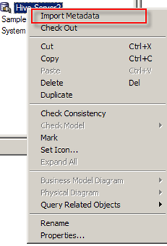
Let’s test the connection, this is done by right clicking on the connection pool and selecting import Metadata

clip_image001

If the connection is successful, the Import Metadata window is displayed

clip_image003

Click Next

clip_image005

For some reason, the hive tables are not listed under the “default” database; click on the shuttled icon then Finish.

The Physical catalog HIVE is created under the Hive Server2 connection pool

clip_image006

We need to create the “crime” table manually in OBIEE. This is done by right clicking on the “HIVE” physical catalog->New Object->Physical Table

clip_image007

The key thing to note is that the table name (CRIME) and the physical columns must match those in the hive database.

image

We then create 2 aliases then a business model in order to be able to create simple interactive reports in OBIEE Answers.


image


We also create a simple measure: count of ID to represent the number of crime occurrences.


image


We’re now ready to create a simple report in OBIEE, the first report will show the # of crime occurrences versus year (2001 through 2015). As soon as the job is submitted, we can log into Spark UI to monitor the job. Sure enough, we see one job being run


image


After a few seconds, the job completes


image


The results are displayed in OBIEE.


image


We then add the crime type in a pivot table


image


We add a tree map visualization to display the number of crime occurrences by crime type for 2015


image


In this post, we connected OBIEE to Hive integrated with Spark SQL; we then created analysis using the Hive-Spark data source.

Monday, April 20, 2015

Exploring geospatial information from the Chicago crime dataset using Apache Spark

In a previous blog post, we experimented with a dataset dealing with crime in Chicago. I’ve been reading a great book “Advanced Analytics with Spark”, I decided to experiment with the techniques that I learned in Chapter 8 in order to analyze the spatial features of the data set. Recall that the crime data set was released by the city of Chicago and made available on the Socrata website. The file has been exported as CSV and is about 4 Gb big;  it contains about 4 million crimes covering the 2001-2014 period. The main question we will try to answer is : what is the spatial distribution of crimes committed?

Let’s start a new IntelliJ IDEA SBT project

image

The SBT build file is

name := "crimeData"

version := "1.0"

libraryDependencies += "org.apache.spark" % "spark-core_2.10" % "1.3.0"

libraryDependencies += "org.apache.spark" %% "spark-sql" % "1.3.0"

libraryDependencies += "com.github.nscala-time" %% "nscala-time" % "0.4.2"

libraryDependencies += "com.esri.geometry" % "esri-geometry-api" % "1.1.1"

libraryDependencies += "io.spray" %% "spray-json" % "1.3.1"

It includes extra dependencies that will be useful for our analyses:


  • nscala-time makes it easy to deal with temporal data computations
  • esri-geometry-api will help with geolocation analyses
  • spray library for handling JSON data

Following the steps covered in previous posts, we’ll create a Resilient Distributed Dataset (RDD) from our CSV dataset. The data will pull be loaded via a Scala case class


  case class crimeData(caseNum:String, id: String,
dateofOcc: DateTime,block: String,IUCR:String,primaryType: String, desc: String,
location: String, arrest: Boolean,domestic: Boolean, beat: String,
district: String, ward: String, community: String, fbiCode: String,xCoord: Long,
yCoord: Long, year: Int, updatedOn: DateTime,lat: Double, lon: Double, loc: String,crimeCoord: Point)

One noteworthy detail is the type of the last field crimeCoord: Point. This attribute from the ESRI geolocation API will store the GPS coordinates where the crime occurred, it is define as “a  single location in space and is the building block for all other geometry types”. Using this field and additional operations provided by the ESRI API, we will be able to determine for a given Point in space, where it is located in the city of Chicago.


  def point(longitude: String, latitude: String): Point = {
new Point(longitude.toDouble, latitude.toDouble)
}

The spatial data used for the boundaries of the different areas of Chicago is in a format called GeoJSON which is  an open standard format for encoding collections of simple geographical features along with their non-spatial attributes using JSON. The main objects of GeoJSON are Point and feature made up of a geometry instance and a set of key-value pairs called properties.A geometry is a shape like a point, line, or polygon. A set of features is called a FeatureCollection. . The Chicago GeoJSON dataset used for this analysis is available here.


image.


Let’s write our parsing function, we will use a slightly different approach this time by making use of Scala Either class which represents a value of one of two possible types Instances of Either are either an instance of scala.util.Left or scala.util.Right: Either[L,R] In the context of the CSV file parsing, the “left” output will represent data successfully parsed and the “right” output will be a tuple of the exception and the data that caused it. The original code for parsing the records is in the “Advanced Analytics with Spark” book, the listing is a follows:


def safe[S, T](f: S => T): S => Either[T, (S, Exception)] = {
new Function[S, Either[T, (S, Exception)]] with Serializable {
def apply(s: S): Either[T, (S, Exception)] = {
try {
Left(f(s))
} catch {
case e: Exception => Right((s, e))
}
}
}
}

We can now create a safe wrapper function called safeParse by passing our parse function (of type  String=>crime) to the safe function, and then applying safeParse to the crimeRaw RDD. We then print the first 10 records to ensure that our parsing function is working correctly.


val safeParse = safe(parse)
val crimeParsed = crimeRaw.map(safeParse)
crimeParsed.cache()
crimeParsed.take(10).foreach(println)

 image


The first record being the header falls into the “Right” category, the exception is “java.text.ParseException: Unparseable date: "Date" ” the remaining 9 records are valid.


We can apply map to only select the valid records:


  crimeGoodData.values.map(zone).countByValue().foreach(println)

We’ve got our data read in ,cleaned up and read into an RDD, we can proceed with the geospatial analysis: recall that our main goal is to find get a distribution of crime occurrence in Chicago.


The first step is to load our geolocation file using regular Scala IO command


  val geojson = scala.io.Source.fromFile("/home/spark/data/chicago.geojson").mkString

We will be using Spray and Esri into the Spark shell so that we can parse the geoJSON string into an instance of our FeatureCollection case class as illustrated in the book mentioned earlier, the code below is to be inserted into our chicagoCrime object. It contains all the objects needed for processing the geoJSON data and to perform the operations for assigning each crime occurrence into a neighborhood in Chicago.


  class RichGeometry(val geometry: Geometry,
val spatialReference: SpatialReference =
SpatialReference.create(4326)) {
def area2D() = geometry.calculateArea2D()

def contains(other: Geometry): Boolean = {
GeometryEngine.contains(geometry, other, spatialReference)
}
def distance(other: Geometry): Double =
GeometryEngine.distance(geometry, other, spatialReference)
}
object RichGeometry {
implicit def wrapRichGeo(g: Geometry) = {
new RichGeometry(g)
}
}

case class Feature(
val id: Option[JsValue],
val properties: Map[String, JsValue],
val geometry: RichGeometry) {
def apply(property: String) = properties(property)
def get(property: String) = properties.get(property)
}

case class FeatureCollection(features: Array[Feature])
extends IndexedSeq[Feature] {
def apply(index: Int) = features(index)
def length = features.length
}

case class GeometryCollection(geometries: Array[RichGeometry])
extends IndexedSeq[RichGeometry] {
def apply(index: Int) = geometries(index)
def length = geometries.length
}

object GeoJsonProtocol extends DefaultJsonProtocol {
implicit object RichGeometryJsonFormat extends RootJsonFormat[RichGeometry] {
def write(g: RichGeometry) = {
GeometryEngine.geometryToGeoJson(g.spatialReference, g.geometry).parseJson
}
def read(value: JsValue) = {
val mg = GeometryEngine.geometryFromGeoJson(value.compactPrint, 0, Geometry.Type.Unknown)
new RichGeometry(mg.getGeometry, mg.getSpatialReference)
}
}

implicit object FeatureJsonFormat extends RootJsonFormat[Feature] {
def write(f: Feature) = {
val buf = scala.collection.mutable.ArrayBuffer(
"type" -> JsString("Feature"),
"properties" -> JsObject(f.properties),
"geometry" -> f.geometry.toJson)
f.id.foreach(v => { buf += "id" -> v})
JsObject(buf.toMap)
}

def read(value: JsValue) = {
val jso = value.asJsObject
val id = jso.fields.get("id")
val properties = jso.fields("properties").asJsObject.fields
val geometry = jso.fields("geometry").convertTo[RichGeometry]
Feature(id, properties, geometry)
}
}

implicit object FeatureCollectionJsonFormat extends RootJsonFormat[FeatureCollection] {
def write(fc: FeatureCollection) = {
JsObject(
"type" -> JsString("FeatureCollection"),
"features" -> JsArray(fc.features.map(_.toJson): _*)
)
}

def read(value: JsValue) = {
FeatureCollection(value.asJsObject.fields("features").convertTo[Array[Feature]])
}
}

implicit object GeometryCollectionJsonFormat extends RootJsonFormat[GeometryCollection] {
def write(gc: GeometryCollection) = {
JsObject(
"type" -> JsString("GeometryCollection"),
"geometries" -> JsArray(gc.geometries.map(_.toJson): _*))
}

def read(value: JsValue) = {
GeometryCollection(value.asJsObject.fields("geometries").convertTo[Array[RichGeometry]])
}
}
}

Now that all the requisite objects are defined for parsing geoSON, let’s process our geoJSON data file into an instance of our FeatureCollection case class.


  val features = geojson.parseJson.convertTo[FeatureCollection]

FeatureCollection contains a function “find’ that will allows to find to what part of Chicago from the geoGSON file a given point where a crime occurred belongs to.


  def zone(crime: crimeData): Option[String] = {
val feature: Option[Feature] = features.find(f => {
f.geometry.contains(crime.crimeCoord)
})
feature.map(f => {
f("name").convertTo[String]
})
}


Finally, we can process crimeDataGood to get a list of Chicago neighborhoods and the associated number of crimes ordered descending ; this is achieved by using sortBy(-_._2)


crimeGoodData.values.map(zone).countByValue()
.toList.sortBy(-_._2).foreach(println)

image


How about the number of crimes type “Homicide” per neighborhood?


    crimeGoodData.values.filter{ p =>
p.primaryType=="HOMICIDE"
}.map(zone)
.countByValue()
.toList.
sortBy(-_._2)
.foreach(println)

image


The code is available here.

Friday, March 13, 2015

Reading Oracle data using the Apache Spark DataFrame API

The new version of Apache Spark (1.3) introduces a new API, the DataFrame. As mentioned in an earlier post, the new API will make it easy for data scientists and people with a SQL background to perform analyses with Spark.

The goal of this post is to experiment with the jdbc feature of Apache Spark 1.3. We will load tables from an Oracle database (12c) and generate a result set by joining 2 tables.

In order to connect to the database using JDBC, a JAR file has to be added to our CLASSPATH. The ojdbc JAR is available at

http://www.oracle.com/technetwork/database/features/jdbc/jdbc-drivers-12c-download-1958347.html

We’ll be using the file ojdbc7.jar.

First download the last Apache Spark 1.3 snapshot from https://spark.apache.org/downloads.html

image

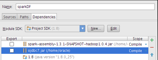
We create a new project in IntelliJ idea then add the Spark 1.3 jar and the ojdbc7.jar file to our project as a dependency under “Project Structure”, “Modules”

image

Oracle databases come with several seed schemas such the HR, we’ll pull 2 tables from that schema: EMPLOYEES and DEPARTMENTS.

image

image

To connect to the Oracle database, the JDBC thin driver will be used. Given the following:

    • Database server: localhost
    • Database service name: pdborcl
    • Port:  1521
    • Userid/password: hr/hr

the JDBC URL is

jdbc:oracle:thin:hr/hr@//localhost:1521/pdborcl

Let’s create a DataFrame (employees) from the “EMPLOYEES” table of the Oracle database:


  val employees = sqlContext.load("jdbc", 
Map("url" -> "jdbc:oracle:thin:hr/hr@//localhost:1521/pdborcl",
"dbtable" -> "hr.employees"))

and a second DataFrame from the “DEPARTMENTS”


val departments  = sqlContext.load("jdbc", 
Map("url" -> "jdbc:oracle:thin:hr/hr@//localhost:1521/pdborcl",
"dbtable" -> "hr.departments"))

Let’s join EMPLOYEES and DEPARTMENTS and print out the results


   val empDepartments = employees.join(departments, 
employees.col("DEPARTMENT_ID")===
departments("DEPARTMENT_ID"))

image


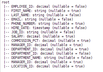
The new DataFrame API has a nice function (printSchema) that prints out the DataFrame schema in a nice tree format.


 empDepartments.printSchema()

image


Following is the whole code listing


import org.apache.spark.sql.SQLContext
import org.apache.spark.{SparkContext, SparkConf}
object sparkJDBC {
def main(args: Array[String]): Unit = {
val conf = new SparkConf().setAppName("ORCL db")
.setMaster("local[4]")
val sc = new SparkContext(conf)
var sqlContext = new SQLContext(sc)
val employees = sqlContext.load("jdbc",
Map("url" -> "jdbc:oracle:thin:hr/hr@//localhost:1521/pdborcl",
"dbtable" -> "hr.employees"))
val departments = sqlContext.load("jdbc",
Map("url" -> "jdbc:oracle:thin:hr/hr@//localhost:1521/pdborcl",
"dbtable" -> "hr.departments"))
val empDepartments = employees.join(departments,
employees.col("DEPARTMENT_ID")===departments("DEPARTMENT_ID"))
empDepartments.foreach(println)
empDepartments.printSchema()
}
}


There you have it, this was a quick introduction to using the new Apache Spark DataFrame JDBC feature to pull data from an Oracle database. This new API will without a doubt offer more flexibility to perform analyses stored in a relational database.

Saturday, February 21, 2015

Experimenting with the Apache Spark Dataframe API

The goal of this post is to experiment with a new introduced a new Apache Spark API: the dataframe. It makes it easier for data scientist to manipulate data. This feature will be part of Apache Spark 1.3 due to be released early March, however one can download the development branch and build it.

I will be experimenting with a Chicago crime data set from www.socrata.com. The file can be downloaded from chicagoCrimeData.csv

image

The data set includes a header and it contains 10 fields

Case# Date Block Primary Desc Secondary Desc Location Desc Arrest Domestic Latitude Longitude
String String String String String String String String Double Double

The second field will be split into two: date and time. Following is the case class that will be used to load the data

case class crimeData(caseNum: String, date: String, time: String, block: String,
primaryDesc: String, secondaryDesc: String, location: String, arrest: String,
domestic: String, lat: String, lon: String)

Prior to parsing the data, we need to set filters for removing the header as well as taking care of missing data. Lines that include missing data for a given field represented by “,,” will be excluded


    val input = sc.textFile(filename)
val data = input.filter(line => !line.contains(",,"))
val header = data.take(1)(0)
val goodData = data.filter(line=> line != header)

We can define a method for parsing the different fields


    def parseCrimeData(str: String): crimeData = {
val fields = str.split(",")
crimeData(fields(0), fields(1).split(" ")(0), fields(1).split(" ")(1), fields(2), fields(3), fields(4), fields(5),
fields(6), fields(7), fields(8), fields(9))
}
We then load the data by
val crime = goodData.map(parseCrimeData)

Once the data is loaded, we can print it out to make sure that our parsing method worked properly


image


Now that we’ve got our crime RDD, we can use the method toDF() in order to convert our RDD into a data frame crimeDF


val crimeDF = crime.toDF()

The data frame will allow us to perform data analysis in a flexible way, let’s get a count of the crime occurrences by crime type. This is easily done by:


crimeDF.select( "caseNum", "primaryDesc").orderBy("primaryDesc").groupBy("primaryDesc").count().distinct.foreach(println)

image


One of the nice feature of a Spark data frame is that it allows running regular SQL against it after the DF has be registered as a temporary table (crimeData)


crimeDF.registerTempTable("crimeData")

Let’s run the same query as the previous query but by using a regular SQL query:


    sqlContext.sql(
"""
|SELECT count( distinct caseNum), primaryDesc
| FROM crimeData group by primaryDesc
| order by primaryDesc
""".stripMargin)
.collect()
.foreach(println)

we get a tabulation of crimes by crime type


image


Following is the full code listing


import org.apache.spark.sql.SQLContext
import org.apache.spark.{SparkConf, SparkContext}
case class crimeData(caseNum: String, date: String, time: String, block: String,
primaryDesc: String, secondaryDesc: String, location: String, arrest: String,
domestic: String, lat: String, lon: String)
object sparkDF {
def main(args: Array[String]) {
val conf = new SparkConf().setAppName("sparkDF").setMaster("local[4]")
val sc = new SparkContext(conf)
val filename = "chicagoCrimeData.csv"
def parseCrimeData(str: String): crimeData = {
val fields = str.split(",")
crimeData(fields(0), fields(1).split(" ")(0), fields(1).split(" ")(1), fields(2), fields(3), fields(4), fields(5),
fields(6), fields(7), fields(8), fields(9))
}
val sqlContext = new SQLContext(sc)
import sqlContext.implicits._
val input = sc.textFile(filename)
val data = input.filter(line => !line.contains(",,"))
val header = data.take(1)(0)
val goodData = data.filter(line => line != header)
val crime = goodData.map(parseCrimeData).toDF()
val crimeDF = crime.toDF().cache()
crimeDF.select( "caseNum", "primaryDesc").orderBy("primaryDesc").groupBy("primaryDesc").count().distinct.foreach(println)
crimeDF.registerTempTable("crimeData")

sqlContext.sql(
"""
|SELECT count( distinct caseNum), primaryDesc
| FROM crimeData group by primaryDesc
| order by primaryDesc
""".stripMargin)
.collect()
.foreach(println)
}
}

Monday, February 16, 2015

Building Apache Spark 1.3 development branch

In this short post, I am documenting how to download and build Apache Spark development branch 1.3 in Linux Mint. Apache Spark 1.3 provides a new feature, the DataFrame API similar to that of R and to a database table. The official version 1.3 is due to be released in early March, however one can download and evaluate the development version.

To download and build Apache Spark 1.3, do the following:

* clone the 1.3 branch by running at the shell prompt

git clone -b branch-1.3 https://github.com/apache/spark.git

image


Once this step is done, there should be a folder called “spark”, cd into the folder then run the build command using sbt


sudo sbt/sbt assembly


After a while, if the build is successful, you’ll see


image


the Spark shell is started by running the following command


 bin/spark-shell 


image

Thursday, January 22, 2015

Visualizing a data set in Spark

The goal of this post is to introduce a nice tool Wisp by Quantifind that enables visualizing data stored in Scala using the web browser. In a previous post, we loaded a weather data set into an RDD. To include Wisp in the project, update the sbt definition and add:

libraryDependencies += "com.quantifind" %% "wisp" % "0.0.1"

We’re going to plot the averages of


  • tMinimum
  • tAverage
  • tMaximum

for all years.


The averages will be stored in mutable lists


    var tempAverage = new ListBuffer[Double]
var tempMinimum = new ListBuffer[Double]
var tempMaximum = new ListBuffer[Double]


We need to add an import for the Scala mutable list and the Highchart library


import scala.collection.mutable.ListBuffer
import com.quantifind.charts.Highcharts._

The averages are computed using the Spark function “aggregate”


    for(month <- 1 to 12) {
val monthData = tempData.filter(_.month==month)
val tAve = monthData.map(_.tAverage).aggregate((0.0, 0.0))((p, q) => (p._1 + q, p._2 + 1),(p, q) => (p._1 + q._1, p._2 + q._2))
val tMin = monthData.map(_.tMinimum).aggregate((0.0, 0.0))((p, q) => (p._1 + q, p._2 + 1),(p, q) => (p._1 + q._1, p._2 + q._2))
val tMax = monthData.map(_.tMaximum).aggregate((0.0, 0.0))((p, q) => (p._1 + q, p._2 + 1),(p, q) => (p._1 + q._1, p._2 + q._2))
tempMinimum += tMin._1/tMin._2
tempAverage += tAve._1/tAve._2
tempMaximum += tMax._1/tMax._2
}
The aggregate function provides a  customized way to perform reductions and aggregations with a RDD. In this particular case, aggregate will compute 2 values at the same time

  • sum of the temperature values
  • sum of the number of elements

The ratio of the 2 values represents the average.


Lets’ now use Wisp to plot the temperature profile


   line(1 to 12, tempMinimum)
hold()
line(1 to 12, tempAverage)
hold()
line(1 to 12, tempMaximum)
title("Temperature")
xAxis("Month")
yAxis("Temperature")
legend(List("Tminimum", "Taverage","Tminimum"))

Compile the code and run it, if all goes well, the console displays a URL


Output written to http://machine-name:PORT

Navigate to the URL using a web browser and you should see a chart showing the monthly temperature averages for tMinimum, tAverage and tMaximum.


image

Sunday, December 28, 2014

Loading data using Spark SQL (cont.)

In the previous post we loaded data into Spark via a Scala case class, were continuing our experiment, this time the data will be loaded using Spark SQL. Spark SQL is component of Spark and it provides a SQL like interface.

Continuing with the code from the previous post, let’s create a SQLContext which is an entry point for running queries in Spark

 val sqlContext = new org.apache.spark.sql.SQLContext(sc)
import sqlContext._

Let’s create a schema RDD programmatically, this method is recommended when a case class cannot be defined ahead of time according to the Spark SQL documentation.


There are three steps as detailed in the documentation:


  1. Create an RDD of Rows from the original RDD;
  2. Create the schema represented by a StructType matching the structure of Rows in the RDD created in Step 1.
  3. Apply the schema to the RDD of Rows via applySchema method provided by SQLContext.

The schema RDD is represented by by a StructType matching the structure of the data that is being read.


val schema = StructType(Array(StructField("year",IntegerType,true),
StructField("month",IntegerType,true), 
StructField("tAverage",DoubleType,true),
StructField("tMaximum",DoubleType,true),
StructField("tMinimum",DoubleType,true)))

Next, we convert the rows of the weather data into Rows


val rowRDD = source.map(_.split(","))
  .map(p => org.apache.spark.sql.Row(p(1)
  .toInt,p(2).toInt,p(4).toDouble,p(5)
  .toDouble, p(6).toDouble ))

Next, we apply the schema


val tempDataRDD = sqlContext.applySchema(rowRDD, schema)

Finally we register the schema as a table


tempDataRDD.registerTempTable("temperatureData")

Now that the schema has been registered, we can run a SQL query


sql("select year, month, AVG(tAverage) 
  from temperatureData group by year order by 
  year").foreach(println)

to compute the average temperature by year. The results are displayed interleaved with log entries


image


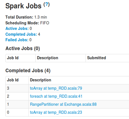
Note that while the application is running, you can get all the job details by logging into sparkUI, typically the port is 4040 (the correct port is displayed on the console)


image


image